Introduction to Central Limit Theorem

Author

Jose Toledo Luna

library(palmerpenguins)

Sampling Distributions

Sample mean

The sampling distribution of the sample mean is the theoretical distribution of means that would result from taking all possible samples of size $n$ from the population.

Suppose we are sampling from a population which comes from a standard Normal distribution such that observations in our sample are iid (independent, identically distributed). Each sample of size $n$ will then consists of realizations $\{x_1,\dots,x_n\}$, such that each $x_i$ will be a realization of the random variable $X_i \sim N(0,1)$

To obtain the sampling distribution for the sample mean,

For the total number of samples do the following:

Generate a random sample of size $n$ from the population
Compute the sample mean and store the result in a variable, say sample_means
Plot each of the sample_means using a histogram

n_samples <- 10000
sample_size <- 100 # each sample will be of size 100
sample_means <- numeric(n_samples)

for(i in 1:n_samples){
  sample_i =  rnorm(n = sample_size, mean = 0, sd=1) # generate a new sample
  sample_means[i] = mean(sample_i) # obtain mean for each sample
}

Then simply use hist(sample_means) to visuallize the distribution with a histrogram.

Show Code (optional)

The sampling distribution of the sample mean, using ggplot2

sampling_dist <- ggplot(data.frame(sample_means),aes(sample_means))+
  geom_histogram(fill = 'steelblue',alpha = 0.3,
                 color = 'black',bins=30)+
  labs(title = 'Sampling distribution',
       x = 'Sample means',y = '')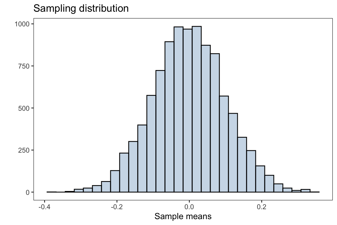

The plot above is the distribution of sample means after taking 10,000 samples with size $n=100$ from the population. The overall distribution appears to be normally distributed (bell shaped curve).

The Central Limit Theorem (CLT) states that if you have a population with mean $\mu$ and standard deviation $\sigma$ and take sufficiently large random samples from the population with replacement, then the distribution of the sample means (sampling distribution) will be approximately normally distributed with mean $\mu$ and standard error $\frac{\sigma}{\sqrt{n}}$. Note, the standard deviation of the sampling distribution of the sample mean (or any other statistic) is referred to as the standard error.

Recall, the population is distributed as a standard normal distribution, i.e $N(\mu=0,\sigma=1)$

mean(sample_means)

#> [1] -0.0007463523

which is very close to the population mean of $\mu =0$

with standard error

sd(sample_means)

#> [1] 0.1006968

which is approximately $\frac{\sigma}{\sqrt{n}} = \frac{1}{10}$

Below is a demonstration of how increasing the sample size affects the distribution of the sample mean and seeing CLT in action

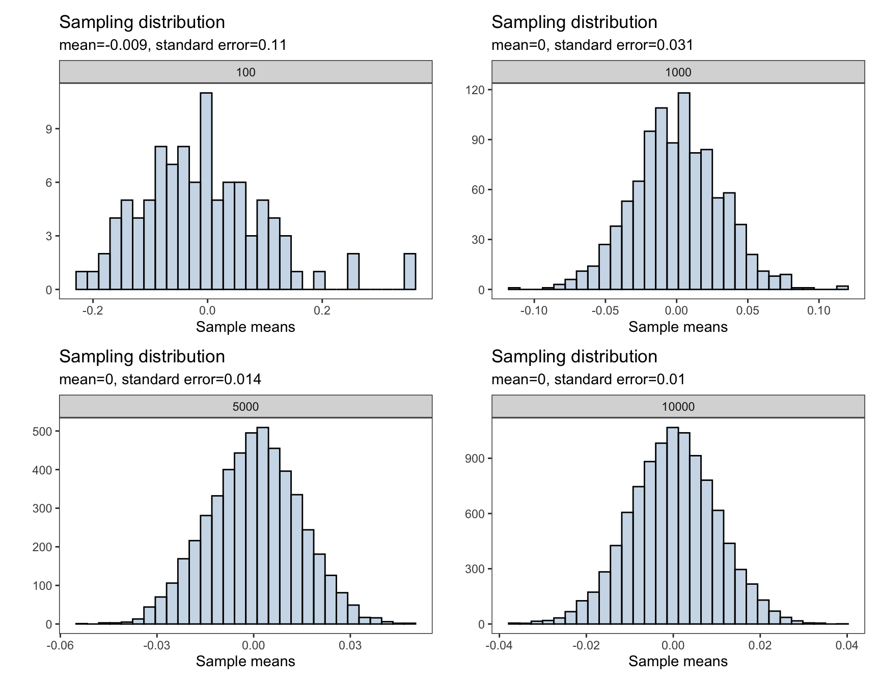
To interactively visualize how the sampling distribution of the sample mean builds up one sample at a time and see when the Central Limit Theorem start to kick in, I highly recommend the art of stats sampling distributions and Central Limit Theorem web applications.

Application: Sample Mean

Now we will apply the the concepts of generating a sampling distribution for the sample mean using a real world dataset. In particular, we will use the penguins dataset from the palmerpenguins package.

Using the penguins dataset we will generate a sampling distribution for the sample mean of the penguins’ body mass (grams)

For simplicity, we will remove any missing observations

body_mass_g <- na.omit(penguins$body_mass_g)

Recall, to obtain the sampling distribution for the sample mean, do the following process

For the total number of samples do the following:

Generate a random sample of size $n$ from the population, penguins$body_mass_g
Compute the sample mean of the penguins body mass and store the result in a variable, say body_mass_xbar
Plot each of the body_mass_xbar using a histogram

n_samples <- 10000
sample_size <- 50

body_mass_xbar <- numeric(n_samples)

for(i in 1:n_samples){
  sample_i =  sample(body_mass_g, size = sample_size) # generate a new sample
  body_mass_xbar[i] = mean(sample_i) # obtain mean for each sample
}
# hist(body_mass_xbar)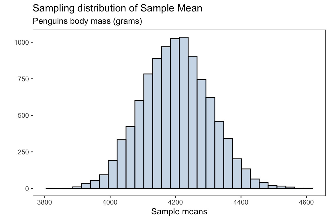

The mean for the sampling distribution is

mean(body_mass_xbar)

#> [1] 4201.383

which is approximately the population mean for the penguins body mass (without missing observations)

mean(body_mass_g)

#> [1] 4201.754

the standard error for the sampling distribution is

sd(body_mass_xbar)

#> [1] 104.3452